Flow of a Viscous Fluid between Dilating and Squeezing Channel: A Model for Biological Transport
Syed Tauseef Mohyud-Din, Naveed Ahmed, Umar Khan
Syed Tauseef Mohyud-Din*, Naveed Ahmed, Umar Khan
Department of Mathematics, Faculty of Sciences, HITEC University, Taxila Cantt, Pakistan.
Received Date: April 16, 2016; Accepted Date: May 05, 2016; Published Date: May 12, 2016
Citation: Mohyud-Din ST, Ahmed N, Khan U. Flow of a Viscous Fluid between Dilating and Squeezing Channel: A Model for Biological Transport. Electronic J Biol, 12:4
Abstract
In the study of fluid transport in biological organisms, we deal with the flow between permeable walls that may expand or contract, this type of flow has a great importance in medical and biological sciences. In this article, the laminar flow of an incompressible viscous fluid is considered in a semi-infinite rectangular domain. It is bounded by two moving porous walls that enable the fluid to enter or exit during successive contractions or expansions. The solution of the problem is approximated by using Variation of Parameters Method (VPM). To investigate the effect of non-dimensional wall expansion/contraction rate and permeation Reynolds number, on the flow field, the graphical results are presented. A couple of graphs, highlighting the effects of involved parameter on the normal pressure distribution, are also included. The analytical solution obtained by (VPM) is also supported by numerical results and both show an excellent agreement. A comparison among the current solution and some already existing solutions is also presented. The study of the flow between dilating or squeezing porous walls is drastic simplification of the transport of biological fluids through dilating or squeezing vessels.
Keywords
Fluid transport; Biological transport.
1. Introduction
In biological fluid transport, the flow through expanding and contracting porous vessels is a common phenomenon. Its vital importance in many parts of synthetic respiratory systems, artificial circulatory systems and several industrial processes is also an established fact. Therefore, its study has attracted many researchers from all over the world and they have contributed their work in this regard.
The pioneer work concerning the steady flow solutions in channels with porous boundaries has been done by Berman [1]. He introduced a method to reduce Navier Stokes equations into a single ordinary differential equation on the basis of the assumption that the suction or injection through the porous bodies is uniform. His study opened a new door for many researchers who later worked on the guidelines provided by him.
Goto and Uchida [2] discussed the effect of viscosity and pressure distribution as well as the effect of wall contraction and realistic length of the body. Governing equations were reduced to a single ordinary differential equation by using similarity transform in time and space. Majdalani [3,4] studied the viscous flow driven by small wall contractions and expansions of two weakly permeable walls by using the same similarity transformation.
Boutros et al. [5] presented Lie-group method solution for two-dimensional viscous flow inside a rectangular domain with slowly expanding or contracting weakly permeable walls. Lie-group method has been applied to reduce the governing partial differential equation by determining reduction symmetric transforms. Many other studies have also been carried out to determine more accurate and easier methods to compute solutions. Mahmood et al. [6] and Asghar et al. [7] have considered the same problem and have done some improvements to the solutions obtained by previous authors.
Upon the aforementioned studies, the present work discusses a more reliable, accurate and feasible solution. We consider an incompressible, laminar, isothermal flow inside a channel having infinite length and use the so called exact similar transform in both space and time to reduce the governing equation of the flow and then solve it with a very effective technique called variation of parameters method (VPM) and it is observed that the results obtained by the VPM are more accurate and provide such results which are nearer to numerical simulation. Visibly low percentage error is observed compared to the works done by Majdalani et al. [4] and Boutros et al. [5]. One may also observe from our work that the VPM is less laborious and gives more accurate results as compared to methods previously used. It also does not require imposing assumption of weak permeable walls which was necessary in many prior studies
2. Formulation of the Problem
In this study, laminar, incompressible and isothermal flow is considered in a rectangular duct of infinite length [8], which contains two permeable walls, from where the fluid can enter or exit during successive expansions/contractions. The aspect ratio of the width W to the height 2α of the duct is taken to be sufficiently large so that the effect of lateral walls can be ignored; it is normally taken as  [9].
[9].
The head end of the duct is closed with an impermeable, solid membrane that is capable to expand or contract with the dilating or squeezing walls. Due to the higher aspect ratio between the height and the width of the duct we can confine the whole problem to half domain and a plane cross section of the simulated domain as shown in Figure 1.

Figure 1: Two-dimensional domain with expanding or contracting porous walls
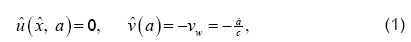
Both walls are assumed to have equal permeability and to expand uniformly at a time dependent rate  The flow is only due to suction or injection, and at the walls the suction or injection velocity −vw is assumed to be independent of position. This enables us to assume flow symmetry about
 The auxiliary conditions for this problem are specified as
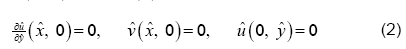
 and
and  here are the velocity components in
  and
and  -directions, respectively, and c is the suction coefficient which is the measure of wall porosity [2]. For two dimensional, unsteady, incompressible viscous fluid, the equations of continuity and momentum in component form are
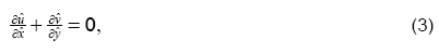
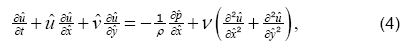

 and t are the dimensional pressure, density, kinematic viscosity and time, respectively.
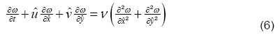
We can simplify the above system of equations by eliminating the pressure terms from, Eqs. (4) and (5). After cross differentiation, using Eq. (3), and introducing vorticity ω we get
with,

Due to the conservation of mass, a similar solution can be developed with respect to as follows,

where,  represents
Using Eq. (8) in Eq. (7), we get
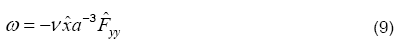
Substituting Eq. (9) in Eq. (6), we obtain
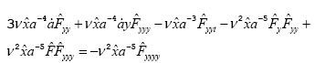
A careful simplification leads to,
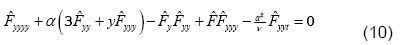
while,  is non-dimensional wall expansion or contraction rate, taken to be positive for expansion.
The auxiliary conditions can also be transformed as

R here is the permeation Reynolds number defined as  it is taken to be positive for injection.
We can now obtain  by setting α to be a constant or a quasi-constant in time [3]. The value of the expansion ratio α in this case can be specified by its initial value
where, a0 and  represent the initial channel height and expansion rate, respectively.
Integrating, Eq. (12), with respect to time; a similar solution for temporal channel altitude evolution can be determined and is given by
3. Dimensionless form of the Governing Equations
Eq. (8), Eq. (10) and Eq. (11) can be made non-dimensional by introducing non-dimensional parameters
Substituting,  in Eqs. and we get


where, ′ denotes differentiation with respect to y .
We solve Eq. (14) subject to the boundary conditions, provided in Eq. (15), using Variation of Parameters Method (VPM) which has been employed successfully to determine the solution of several research problems [10-13].
4. Variation of Parameters Method
To illustrate the basic concept of the variation of parameters method for differential equations, we consider the following general differential equation in operator form
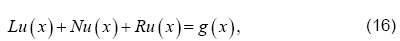
where, L is the highest order linear operator, R is the linear operator of order less than L,N is the nonlinear operator, and g is the source term. We have the following general solution of equation

where, n is the order of given differential equation and  is are the unknowns that can be determined by using the supporting initial/boundary conditions.
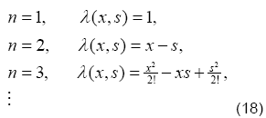
Moreover, λ (x, s) is the multiplier and it is used for the reduction of the order of the integration; it can be determined with the help of Wronskian technique. For different values of order n, one can easily obtain the following values of the multiplier.
The Eq. (17) leads us to an iterative scheme that is given as
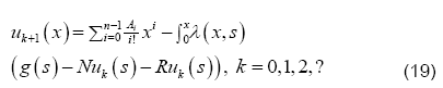
The above iterative algorithm provides us the solution of the differential equation, with sufficient auxiliary conditions, at different levels of iterations. The terms outside the integral, provides us with the initial guess and its presence in all the iterations gives us a better approximation.
5. Application of VPM to the Problem
Following the guidelines provided in above section, Eq. (14) gives us the following iterative scheme,
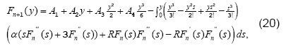
with n = 0,1,2,3?
Utilizing the boundary conditions given in Eq. (15),
we have A1 = 0, A3 = 0. Moreover, by
setting A2 = A, , and A4 = B , Eq. (20) leads us to,
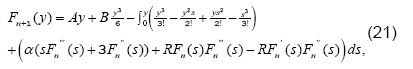
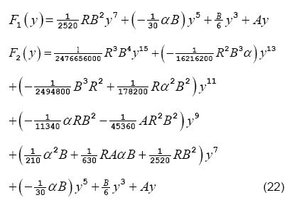
First two iterations of the solution are given as
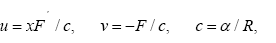
As we have found the pivotal variable F, the normal pressure distribution can be expressed as a function of F. The desired expression can be obtained by substituting Eq. (8) into the Eq. (5) and using  The consequent result is as follows
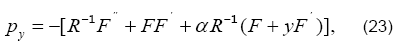
Where  denotes the dimensionless pressure. The normal pressure distribution now can readily be determined by integrating Eqn. (23) with respect to y and letting pc to be the central line pressure.

After a careful manipulation, we get
which is the expression for the normal pressure distribution 
6. Results and Discussion
After the successful determination of F; we can find the other flow characteristic in terms of F. The graphical representation of the flow behavior is an easy way to see the effects of different flow parameters on the flow field; the figures to follow are displayed for the same purpose. Over the range of non-dimensional wall expansion/contraction rate α, Figures 2 and 3, show the behavior of axial velocity, F' (or uc/x, for the permeation Reynolds numbers, R=3 and R=−3 , respectively. It can clearly be seen with increasing value of α, the expansion (α > 0) combined with, suction or injection, delays the flow near the walls; however it rises the fluid’s velocity near the centreline of the channel. In fact, the expansion of the walls creates a space nearby; to fill it, the fluid in the vanicity moves in; in a result, a delayed axial flow near the walls is as expected. The phenomenon is least dominant near the center, so the conservation of mass ensures an increased axial flow there.

Figure 2: Effects of wall deformation rate on axial velocity in case of injection.

Figure 3: Effects of wall deformation rete on axial velocity in case of suction.
On the other hand, when the contraction (α > 0) is combined with suction or injection, the increasing absolute value of α decrease the axial velocity near the walls; however, at the center, the behavior is opposite and an accelerated flow is observed for increasing |α|. The contraction hinders the axial flow near the walls and hence a velocity-drop there is expected. Moreover, it leads to a heavier flow near the center and hence an accelerated flow near the center is also logical. From the same figures it can be concluded that the deviations in the velocity are more prominent in the case of suction (R=−3). The maximum of the velocity lies near the center in all these cases; it decreases with increasing expansion and does the otherwise for increasing contraction.
Figures 4 and 5 show the behavior of axial velocity F′ ( or uc / x) over the range of permeation Reynolds numbers R; the wall deformation rate is taken to be α = 2.5 and α = −2.5 , respectively. Figure 4 depicts, in case of expansion, the increasing R; leads to a decelerated flow near the walls and acceleration near the centerline of the channel. Figure 5 on the other hand shows a quite opposite behavior, in case of contraction, there is a slight increase in the velocity near the walls with increasing R and near the centerline the same decrease. It can also be seen that these two figures affirm the results obtained in Figures 2 and 3.

Figure 4: Effects of permeation Reynolds number on axial velocity in case of expansion.

Figure 5: Effects of permeation Reynolds number on axial velocity in case of contraction.
To support our analytical work future, we have solved Eq. (14) with Eq. (15) numerically by using the shooting method combined with fourth order Runge- Kutta scheme. A comparison between the numerical solution and the purely analytical solution, obtained by VPM, is presented in Figures 6 and 7. The solution is given for the axial velocity for the cases of contraction combined with injection (Figure 6) and the expansion coupled with injection (Figure 7). It is evident from the figures that the solution obtained by VPM has a remarkable agreement with the numerical solution. Numerical values for the velocity profile are given in Tables 1 and 2.

Figure 6: Comparison between numerical and analytical solution (expansion/injection).

Figure 7: Comparison between numerical and analytical solution (contraction/injection).
| y | VPM | Numerical | [4] | [5] | %error(VPM) | %error [4] | %error [5] |
|---|---|---|---|---|---|---|---|
| 0 | 1.557560 | 1.559473 | 1.536002 | 1.556324 | 0.122669 | 1.515606 | 0.212613 |
| 0.1 | 1.539048 | 1.540888 | 1.519377 | 1.538164 | 0.119411 | 1.396013 | 0.176781 |
| 0.2 | 1.483882 | 1.485503 | 1.469505 | 1.483935 | 0.109121 | 1.076941 | 0.105553 |
| 0.3 | 1.393173 | 1.394434 | 1.386445 | 1.394421 | 0.090430 | 0.572920 | 0.000932 |
| 0.4 | 1.268770 | 1.269540 | 1.270464 | 1.271006 | 0.06065 | 0.072782 | 0.115474 |
| 0.5 | 1.113244 | 1.113402 | 1.122275 | 1.115778 | 0.014190 | 0.796926 | 0.213400 |
| 0.6 | 0.929856 | 0.929302 | 0.943364 | 0.931656 | 0.059614 | 1.513178 | 0.253308 |
| 0.7 | 0.722502 | 0.721169 | 0.736373 | 0.722523 | 0.184838 | 2.108243 | 0.187750 |
| 0.8 | 0.495575 | 0.493513 | 0.505538 | 0.493322 | 0.417820 | 2.436612 | 0.038702 |
| 0.9 | 0.253585 | 0.251330 | 0.257149 | 0.250109 | 0.897226 | 2.315282 | 0.485815 |
| 1 | 0 | 0 | 0 | 0 | 0 | 0 | 0 |
Table 1. Comparison among numerical, VPM, Majdalani et al. [3] and Boutros et al. [5] solutions for axial velocity α=0.5 and R=5.0.
| y | VPM | Numerical | [4] | [5] | %error(VPM) | %error [4] | %error [5] |
|---|---|---|---|---|---|---|---|
| 0 | 1.557560 | 1.559473 | 1.536002 | 1.556324 | 0.122669 | 1.515606 | 0.212613 |
| 0.1 | 1.539048 | 1.540888 | 1.519377 | 1.538164 | 0.119411 | 1.396013 | 0.176781 |
| 0.2 | 1.483882 | 1.485503 | 1.469505 | 1.483935 | 0.109121 | 1.076941 | 0.105553 |
| 0.3 | 1.393173 | 1.394434 | 1.386445 | 1.394421 | 0.090430 | 0.572920 | 0.000932 |
| 0.4 | 1.268770 | 1.269540 | 1.270464 | 1.271006 | 0.06065 | 0.072782 | 0.115474 |
| 0.5 | 1.113244 | 1.113402 | 1.122275 | 1.115778 | 0.014190 | 0.796926 | 0.213400 |
| 0.6 | 0.929856 | 0.929302 | 0.943364 | 0.931656 | 0.059614 | 1.513178 | 0.253308 |
| 0.7 | 0.722502 | 0.721169 | 0.736373 | 0.722523 | 0.184838 | 2.108243 | 0.187750 |
| 0.8 | 0.495575 | 0.493513 | 0.505538 | 0.493322 | 0.417820 | 2.436612 | 0.038702 |
| 0.9 | 0.253585 | 0.251330 | 0.257149 | 0.250109 | 0.897226 | 2.315282 | 0.485815 |
| 1 | 0 | 0 | 0 | 0 | 0 | 0 | 0 |
Table 2. Comparison among numerical, VPM, Majdalani et al. [3] and Boutros et al. [5] solutions for axial velocity α=-0.5 and R=5.0.
The effects of varying α, on the normal pressure distribution  , are highlighted in the next two figures. The value of R is taken to be −2 and 2, respectively. It can be observed for every level of suction or injection that the absolute change in
  is the lowest near the central region. For suction,
  increases with increasing contraction as well as expansion. The most deviant behavior is observed near the walls of the channel. On the other hand, for injection, the pressure drop increases with increasing expansion; in the same case, it decreases with increasing contraction.
7. Conclusion
In this work we have examined an isothermal laminar flow of a viscous incompressible fluid in a rectangular domain bounded by two moving permeable walls. We have used Variation of Parameters Method (VPM) to approximate the solution for the equations governing the fluid flow. It is clear from our work that VPM can successfully be applied to highly nonlinear equations like the one we have and the results obtained are encouraging. The results bear a remarkable resemblance with the numerical solution as well as some of the already existing ones. The effects of different flow parameter on the flow behavior are shown with the help of graphs. The purpose of this study is to improve the work done by the previous researchers and it can be seen that we have applied such a technique that is less laborious and flexible to apply yet it gives quite accurate results. As the flow between the expanding/contracting porous walls is a basic model for understanding the complex fluid motion involved in bio-fluid mechanics and other branches of science, hence, this work can help to understand those flow behaviors in more accurate and flexible way.
References
- Berman S. (1953). Laminar Flow in Channels with Porous Walls. Journal of Applied Physics. 24:1232-1235.
- Goto and Uchida. (1990). Unsteady flow in a semi-infinite contracting expanding pipe with a porous wall. Proceeding of the 40th Japan National Congress Applied Mechanics NCTAM-40, Tokyo, Japan.
- Majdalani J, Zhou C, Dawson C. (2002). Two-dimensional viscous flow between slowly expanding or contracting walls with weak permeability. Journal of Biomechanics. 35: 1399-1403.
- Majdalani J, Zhou C. (2003). Moderate-to-large injection and suction driven channel flows with expanding or contracting walls. Journal of Applied Mathematics and Mechanics. 83: 181–196.
- Boutros ZY, Mina B, Abd-el-Malek. (2007). Lie-group method solution for two-dimensional viscous flow between slowly expanding or contracting walls with weak permeability. Applied Mathematical Modelling. 31: 1092-1108.
- Mahmood M, Hossain MA, Asghar S, et al. (2008). Application of homotopy perturbation method to deformable channel with wall suction and injection in a porous medium. International Journal of Nonlinear Sciences and Numerical Simulation. 9:195-206.
- Asghar S, Mushtaq M, Hayat T. (2010). Flow in a slowly deforming channel with weak permeability: An," Nonlinear Analysis. Real World Applications. 11: 555–561.
- Uchida S, Aoki H. (1977). Unsteady flows in a semi-infinite contracting or expanding pipe. Journal of Fluid Mechanics. 52:371-387.
- Dauenhauer EC, Majdalani J. (2003). Exact self-similarity solution of the Navier--Stokes equations for a porous channel with orthogonally moving walls. Physics of Fluids. 15:1485-1495.
- Noor MA, Mohyud-Din ST, Waheed A. (2008). Variation of Parameters Method for Solving Fifth-Order Boundary Value Problems. Applied Mathematics & Information Sciences– An International Journal. 2: 135-141.
- Mohyud-Din ST, Noor MA, Waheed A. (2009).Variation of parameter method for solving sixth-order boundary value problems. Communication of the Korean Mathematical Society. 24: 605-615.
- Mohyud-Din ST, Noor MA, Waheed A. (2009). Modified Variation of Parameters Method for Second-order Integro-differential Equations and Coupled Systems. World Applied Sciences Journal. 6: 1139-1146.
- Mohyud-Din ST, Noor MA, Waheed A. (2010). Variation of parameter method for initial and boundary value problems. World Applied Sciences Journal. 11: 622-639.


Open Access Journals
- Aquaculture & Veterinary Science
- Chemistry & Chemical Sciences
- Clinical Sciences
- Engineering
- General Science
- Genetics & Molecular Biology
- Health Care & Nursing
- Immunology & Microbiology
- Materials Science
- Mathematics & Physics
- Medical Sciences
- Neurology & Psychiatry
- Oncology & Cancer Science
- Pharmaceutical Sciences