Implicit Fox Rabies model with an Asymptotic Computation of Chaos
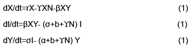
Ippolito A Stephen, Naudot Vincent
Ippolito A Stephen1,*, Naudot Vincent2
1American Seed Trade Association (ASTA), USA;
2Florida Atlantic University (FAU), USA.
Received date: May 13, 2016; Accepted date: August 08, 2016; Published date: August 15, 2016
Citation: Stephen IA, Vincent N. Implicit Fox Rabies model with an Asymptotic Computation of Chaos. Electronic J Biol, 12:4
Abstract
Rabies remains an important human health and wildlife management concern worldwide. Currently, there is significant underreporting of human deaths from rabies in many parts of the world. Concerning foxes in Europe, the proportion of all cases that are observed is likely to be as low as 2−10%. Consequently predictive models have been developed to estimate the mortality attributable to rabies. When rabies penetrates a new area, there is a peak in reported cases among foxes. These pulse like events causing the spread of rabies, often due to migration, mating and other seasonal behaviors are often absent from a rabies model. We present a model which modifies an existing continuous rabies model with the addition of a discrete kick via the Dirac distribution. Furthermore noting the observed complexities in the literature and the data we study the level of complexity of the presented model and use an algorithm to demonstrate the existence of chaos via Taylor expansions and curve fitting for the stable and unstable manifold of a fixed point at the origin.
Keywords
Dynamical systems; Rabies; Chaos.
1. Introduction
Rabies remains an important human health and wildlife management concern worldwide. The presence of rabies in an area exacerbates the uncertainty of conserving rare and threatened mammals [1-15]. The disease is transmitted through the saliva of infected animals and affects the central nervous system. All mammals are thought to be susceptible to this disease and throughout human history it has been one of the most feared of all infectious diseases [4].
Underreporting of human deaths from rabies in many parts of the world is significant [1]. To address problems such as properly estimating the impact of the disease and eliminating it, The World Health Organization’s (WHO) Expert Advisory Panel on Rabies has partnered with entities such as the Bill and Melinda Gates Foundation, the Global Alliance for Rabies Control and the Partnership for Rabies Prevention. Those joint efforts have begun to break the cycle of rabies neglect, and rabies is becoming recognized as a priority for investment [1]. Consequently, methods have been developed to estimate the mortality attributable to rabies. In particular predictive models have been investigated [1]. Modeling offers a relatively inexpensive, way to examine what factors affect rabies transmission as well as management and economics [15]. For instance, modeling techniques have resulted in a revised estimate of the burden of rabies in Africa and Asia [1]. As mentioned, in addition to humans, all mammals may carry the rabies virus. Foxes represent one of the most commonly infected mammals. In the United States and Europe, the proportion of rabies observed in foxes is likely to be as low as 2−10% of the total cases [5,8]. Beyond this the modeling of rabies involves many complex interactions which depend on both space and time dependent aspects demonstrating the need for dynamic models.
Dispersal and competition for fox territories results in an increased chance of encounters in late winter. Also vixen tend to peak in their number of interactions during the summer due to the physiological strain of reproduction. Migration of juvenile foxes, usually in the fall, tends to influence regions of low population density since dispersal distances tend to correlate negatively with population density [8]. If we consider the effects of these interactions we note the observation of interesting dynamics. For instance epidemic cycles of increasing amplitude were described in where each time the disease became epidemic the proportion of infections was increasingly worse [4]. Also in Russia, there are different rabies cycles with foxes and dogs in the same area at the same time [8]. A novel attempt to model fox rabies used a system of Ordinary Differential Equations (ODE’s) where most prior models were computer simulations and statistical models. The model makes an additional contribution by allowing population size to be dynamic. As noted there are times during the year where contact rates are higher, such as when juvenile foxes disperse, or when a neighboring community practices rabies control via culling thereby disrupting the fox’s social structure [4]. Consequently, over a very small time period there may be an increase in the number of infected individuals of a population.
The details of the ODE model in will be explored later on; however, this model does not consider migration [4].
Wildlife rabies emerged in Europe after dog rabies was eliminated, the new primary host being the red fox (V. vulpes) [8]. Coming from the east, fox rabies spread inexorably across the continent within a few decades. By the mid-1980s, large parts of central and western Europe were affected. The westward expansion came to a halt in areas such as France and northern Italy, where foxes were treated with oral rabies vaccine. Infected foxes are responsible for maintaining the rabies virus within the fox population and also for transmission to other wildlife species and domestic animals. In affected areas, rabies is detected in a wide variety of species at different frequencies. To have an idea of what the rabies population dynamics look like, consider Figure 1 below. Here the data presented is from and is comprised of all mammalian species in their database [12]. In Figure 1 the dynamics are dominated by the observed infected red foxes. Recall though, as previously mentioned, that the observations may only represent 2−10% of the total number of red foxes. The data from many countries in Eastern and Western Europe is presented in, however as commonly noted; the Ukraine and the Russian Federation provide a reservoir for spreading the disease to other countries [12]. The countries Belarus and Romania are also shown in Figure 1 to demonstrate the dynamics of nearby countries.
Besides the dynamics presented above, there is also a variety of dynamics present within subpopulations. For instance observed cases within the human population present the dynamics in Figure 2.
Moving further from the Ukraine and the Russian Federation, we see that Western Europe is mostly free from rabies [1,12]. However, they are not free from the threat. Since fox rabies has been controlled in Western Europe, the costs for oral vaccination have been substantially reduced but other European countries now striving to eliminate fox rabies are incurring high costs. Recent incursions into Italy, although now under control, required substantial financial commitments, and costs may escalate elsewhere, given the threat of emergence in countries such as Greece. The cost of setting up a protective barrier along the entire eastern border of the European Union to prevent such incursions is estimated to be over 6 million US dollars per year [8].

Figure 1. Number of observed cases on a yearly basis over all mammalian species. Data taken from [12].

Figure 2. Number of observed cases of rabies in humans on a yearly basis. Data taken from [12].
Consequently understanding the dynamics present in Eastern Europe can be of value to Western Europe as well, allowing better and cheaper control strategies, such as mass vaccination which to date has been the most effective means of control [1].
The data from along with the mentioned space time interaction dependencies indicate that migration has pulse action (Figures 1 and 2) [12]. We will start with the previously described ODE given in and modify it by allowing a periodic influx of infected individuals modeled as a pulse [4].
2. Methods
In section 2.1 it was noted that, for foxes with dominate the spread of rabies, factors such as juvenile migration, seasonal mating and control procedures among countries affect rabies dynamics. These factors do have seasonality however the data presented in Figures 1 and 2 indicates pulse like features, as well. This has encouraged us to model these pulses with a discrete kick. In particular, we consider modifications to the model presented in as given below [4].
2.1 ODE
• Number of Susceptible: X
• Number of Latent: I
• Number of Infected: Y
• Death Rate: b
• Population Growth Rate: a
• Latency Period: 1/σ
• Death Rate of rabid foxes: α
• Rabies Transmission coefficient: β
• Self-competition term related to carrying capacity: γ
• Immigration plus births - Emigration and deaths of susceptible: r
2.2 Adding discrete kicks to an ODE
As already discussed, this model should include some sort of temporal forcing, preferably as a pulse. We accomplish this by modifying equation 1 above as follows:
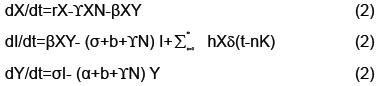
• Dirac distribution: δ
• Time of first instance where infected foxes successfully enter population: k
Dirac distribution δ, defined by the property that
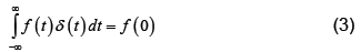
for all continuous functions f defined on R. Equivalently δ may be defined as a probability measure that takes the value of 1 for all sets containing the origin and 0 otherwise [7,11,14].
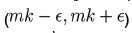
We now show how to integrate (2), however more details can be found in [7]. Let Ia represent the number of latents just after the mth kick and let Ib represent the number of latents just before the mth kick. Thus integrating dI/dt we obtain
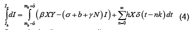
Or equivalently we may write
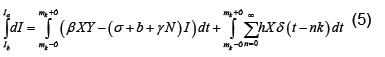
Because 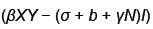 is bounded on
 we have
For  the only non-zero term in the summation is when m=n. Hence, we have
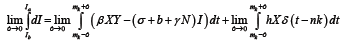 (7)
(7)
which by (6) becomes
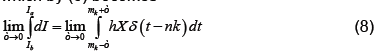
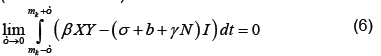
Applying the definition of δ on the right (noting that X is continuous at t=mk) and integrating as usual on the left, which does not depend on ε, we have

In Figure 1 there is a change from few or no to infected animals to populations of considerable size, in the Ukraine. This indicates we are working with introductory level events, particularly of a pulse nature which is modeled by a discrete kick through the Dirac distribution in equation 2. Ideally we consider introductions from each of the classes of the outside environment into the population of study. However, importance in place on the latent class which will become infected and possibly spread the disease rapidly through the study population. We could have modeled the pulse into the infected class; however, rabies has a high death rate. Hence we have worked under the assumption that introduction of the disease through migration is more likely through the latent class.
We consider the pulse action, via the Dirac distribution to be a linear function of the susceptible. Specifically, in the standard epidemic model, the susceptible population determines whether a disease will become an epidemic or die out [10]. The linearity, in the kick term, is to begin simple and avoid over-fitting. A more complex kick term might fit the current data better; however it would also assume more knowledge and may result in increased error when looking at future data. Note that the kick term is a function of the number of susceptible in the population of study when it should be a function of the susceptible in the surrounding populations. This is because we are making an assumption of homogeneity. More precisely we are assuming that the proportion of susceptible in the surrounding populations is proportional to the number of susceptible in the populations of study. It should be noted that by susceptible, latent and infected we are primarily speaking of foxes in the model, however, we may include any mammal.
2.3 Model dynamics
To study the dynamics presented in equation 2 we consider the resulting map at the time of the kick. In particular we integrate equation 1 to the time of a kick and while fixing the values of X and Y, at the said time, we apply equation 9 to the value of I. We may write this map as the composition G=L°XT where L is the kick map and XT is the flow of the ODE at the kick time. Of course since we cannot integrate equation 1 explicitly, the stroboscopic map G does not have an explicit representation. Consequently the dynamics must be studied implicitly. We should also note that in this case G is acting as a hybrid map combining a discrete and a continuous system.
When modeling any system, whether it is to test a hypothesis where we construct a model before fitting it to data, or an observational approach where we construct a model for a particular set of data, we need classes of models which can correctly describe the data. For instance SEIR models, which are a generalization of the model type used in [4], are popular for modeling epidemics. Standard SEIR models, however, typically do not exhibit the complex behavior as is seen in data sets such the 1960’s England and Whales measles epidemic. Consequently, before proposing a class of models we would like to know if a particular class of models can exhibit the necessary dynamics needed to study a system.
A plot representing the dynamics for the map G, with parameters in Table 1, is displayed in Figure 3 below. The reasons for picking these parameters are that rabies seems to exhibit complex dynamics, as discussed in the introduction. Also, from Figures 1 and 2, the dynamics appear to exhibit complexity as well. Consequently, we would like to see if the model presented in equation 2 exhibits complexity, and these parameters are a good place to start.
Proceeding with this investigation note that the map G has a fixed point at X=I=Y=0. If we calculate the Jacobian of the map about this saddle point numerically we find it has a one dimensional unstable manifold and a two dimensional stable manifold, making it hyperbolic. The computed eigenvalues where approximately 5226, 1 × 10⁻⁵ and 1.4 × 10⁻⁸ however for calculations two-hundred decimal places of precision were used. It may be helpful to note that the ratio of the unstable to the stable eigenvalues were about 400 billion and 500 million respectively. Noting the eigenvalues is important not just in terms of identifying a saddle point but the differences in magnitudes indicate how costly a mistake with integration can. Systems such as this are considered stiff and the usual approach is to use integration methods which are A-Stable. The basic idea of A-Stability is to explore the properties of an integration algorithm for a linear model often called the “toy model.” If the region of convergence to 0 for the algorithm is sufficiently large for the product of the step size and the eigenvalue of the toy model, the algorithm is said to be A-Stable. Unfortunately, all A-Stable methods are implicit meaning integration involves solving systems of nonlinear equations. Taylor Integration which was used in this problem is an explicit method that is asymptotically A-Stable, however, which suffices for our purposes (Table 1 and Figure 3) [13].
| ß | s | b | r | Ý | h | k | a |
|---|---|---|---|---|---|---|---|
| 65 | 21 | 1 | 10 | 10 | 7.1 | 23/28 | 13 |
Table 1: Parameter values for used of the model in [2].

Figure 3. Plot of stroboscopic map defined in (2) with parameters defined at this beginning of this section.
2.4 Asymptotic computation of the unstable manifold
The goal for our model is to show the existence of a chaotic set. We do this by showing the transverse intersection of the stable and unstable manifolds for a fixed point, which results in the map represented by our model being conjugate to a horseshoe map and hence containing a chaotic set [9].
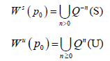
Since the maps we use in our models are implicit we take a numerical approach to estimate the stable and unstable manifolds. We begin by considering an analytic map Q: Rn → Rn and a saddle point p0. The stable manifold theorem guarantees the existence of the local invariant stable and unstable analytic manifolds given by S and U respectively which are tangent to the stable and unstable spaces for DQ (p0) at the said point and of the same dimension. The global stable and unstable sets defined respectively below.
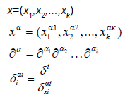
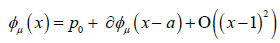
We will discuss the procedure for estimating the unstable manifold; the procedure for the stable manifold is similar. As mentioned above suppose that the dimension of the unstable manifold is given by k ≤ n. Because the manifold is analytic, it has a Taylor expansion about the point p0. So we may parameterize Wu by Taylor expanding about a point a ∈ Rk as below.
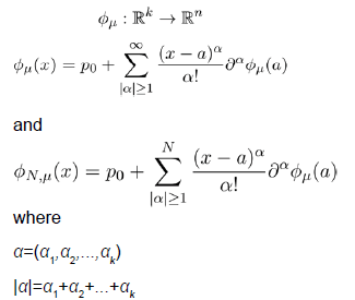
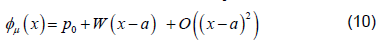
Using the above expansion about  with
with  we may take a linear approximation and write
Since we know that φμ is locally tangent to the unstable Eigen space of DQ (p0), we may write
where 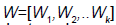 is a matrix of linearly independent columns and
  is an unstable eigenvector of DQ (Su).
Providing a suitable expansion for the unstable manifold would mean knowledge of derivatives beyond the first order which we do not have. Consequently we will use the following property. Let 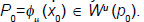 Then we have that for any m0 ∈ N and λ and eigenvalue of DQ (p0).
However convergence is faster when λ−m0x0 << 1, which is the point we will exploit [6]. If Q were a linear map then φμ would just be a matrix consisting of the unstable eigenvectors of DQ (p0) and we could then think of this as the eigenvalue property. Then using a linearization argument, as suggested here, or Normal Form theory we can show that this property holds locally even when Q is not linear. The property can then be extended as a global property of the unstable manifold. To see why this property is useful note that λ gives us information about how quickly points move along the unstable manifold and since λ=1 represents a non-hyperbolic case we would like to stay as far away from this as possible. Consequently we may be better off looking at the map Qm0 and the eigenvalues λm0 if they are more hyperbolic. However, since we are trying to estimate φμthis is just an asymptotic approximation as φN,μ→φ μ .
Specifically we will start with a small neighborhood B0 of points about 0 ∈ Rk. We can then approximate where on the unstable manifold these points should be mapped using equation 11 above writing

We can compute an initial linear approximation for φ0,μ and WμN,m0 using equation 10 then gets a better approximation of the points for the unstable manifold using 11. We then fit WμN,m0 using least squares regression by a polynomial of the desired degree, say N. Since the Taylor expansion of φμ is unique we expect that this regression will approximate , φN ,μ.
Using our estimate of we may use equations 10 and 11 to get a better estimate of  . We repeat this process to show convergence of the polynomial coefficients for ,
3. Results

Figure 4.Considering polynomial fits for the unstable manifold with 200 terms, the above figure shows the change in the coefficients versus algorithm iteration under the L2 norm.
We calculated parameterizations for the unstable and stable manifolds by applying the algorithm in the previous section to our map. Error was calculated for the stable manifold by integrating estimated points forward in time to see if the points converged to the origin. For the unstable manifold points were integrated backwards in time to see if they converged to as well to the origin, which is the saddle point about which we are studying the map. The error for the stable manifold after two iterations was 6 decimals and 40 decimal places for the unstable manifold after 10 iterations. For the unstable manifold the change in regression coefficients with respect to the L2 norm is shown in Figure 4. Noting this is only a Cauchy argument, however, there does appear to be convergence. Only two iterations were performed for the stable manifold. Integrating backwards in time was a computationally difficult task. For the current results 200 terms were needed for Taylor integration, not expansion of the manifolds which also uses Taylor’s theorem 2. Using less terms results in nonsensical output or the system blowing up. Recently work has been done to speed this up using cluster based computing. For Taylor expansions for the actual manifolds only 30 terms were used, for the stable manifold, do to time constraints resulting from computational difficulty and 60 for the unstable manifold (Figure 4).
The output of the algorithm can be viewed in Figure 5. The upper left and right show estimations of the stable and unstable manifolds respectively. The bottom center demonstrates two intersections of the stable and unstable manifold. One intersection occurs at the origin since that is the saddle point. A second intersection occurs by taking a point on the unstable manifold and iterating forward in time. Their intersection which at least from the numerical approximations appear to be transverse indicating conjugacy to a horseshoe map and hence a chaotic set. Thus addressing the question if the model from [4] can be modified to handle the more complex dynamics of rabies models (Figure 5).

Figure 5.Stable and unstable manifolds for the fixed point (0,0,0). Upper lefts is an estimation of the stable manifold. Upper right is an estimation of unstable manifold. Bottom center is an overlay showing the intersection of the stable and unstable manifolds.
4. Discussion
Rabies remains an important problem worldwide. In Western Europe the disease is under control at both the animal and human level, however, maintaining the status quo is expensive [1]. In Eastern Europe such as the Balkans (see Appendix A) the Ukraine and the Russian Federation(Figures 1 and 2) we see that the human cases are relatively under control, while there is still a considerable degree of infection for animal populations, though both are underreported [1]. Still in other parts of the world, such as Africa and parts of Asia neither the human or animal populations are under control [3].
The underreporting is partially why we need modeling. As discussed in the rabies observations only tell us severity relative to other animal populations [3]. Concerning the total numbers of susceptibilities, latent or infected, for any animal or human group we have often have limited information. Rabies, however, spreads between animal species so by modeling we can specify how this information is related, and update the models as new information becomes available. At very least if we cannot give exact numbers for populations we may be able to specify the qualitative dynamics such as cycles or other attractors which can helps us control the spread of this dangerous disease.
As pointed out in the introduction rabies is both a serious problem and one known to exhibit complex dynamics. In a model was developed for the rabies virus and a variable population however the model leaves out migration events that are known to be important to rabies dynamics [4]. For instance, dispersion of juveniles, increased contact during mating season, etc. To account for what from the data seem to be impulse events and likely migration a Dirac distribution was used to introduce a kick and it was assumed to be a function of the number of susceptible in the surrounding community. The assumption is made that the number of susceptible in the community being modeled is proportional to the number of susceptible in surrounding communities. In cases where this assumption is not reasonable, further considerations would have to be made. Also as noted earlier, it is primarily foxes that are being modeled since they are primarily responsible for spreading and maintaining the disease. Starting with a simple pulse to avoid over fitting we observe seemingly complex dynamics [2]. As mentioned earlier, knowing the range of dynamics of a model is important biologically. If the known dynamics of a biological system are known to be more complex than those attainable by that model, then the model should not be used. To study the model’s dynamics, the algorithm in the previous section was used to estimate the stable and unstable manifolds of a fixed point and look at their intersection via curve fitting and Taylor expansion of the manifolds. After running the algorithm the estimations appear to have a transverse intersection. Unfortunately due to stiffness of the ODE the accuracy of the manifolds was only computed to 6 and 40 decimal places for the stable and unstable manifolds respectively. The computation of this intersection reveals chaos and is evidence that this model can mimic the complex dynamics found in nature.
With regards to the algorithm, the accuracy was restricted due to computational limitations. The ratio of the eigenvalues for the unstable to the stable manifolds had an order as high as 400 billion meaning slight errors in the computations can blow up very quickly. This placed restraints on the number of times the algorithm for estimating the manifolds could be used. For the unstable manifold expansion (not Taylor Integration) 60 terms were used and for the stable manifold while 30 were used for the stable manifold. The latter case being two dimensional. Since the main difficulty in the calculation stems from integration of the underlying ODE one option would be to use an integrator other than Taylor’s method with better stability properties or one that takes advantage of resources such as parallel integrators.
For this model to be of use we would like to apply it to the problem is Eastern Europe. However before doing this we may modify the model to include interactions between different species.
Consequently the data from 1977 to 2016 is presented below and shows control of the disease in the human population however demonstrates epidemics for animals, in particular with foxes (Table 2).
| Country | Human | Domestic | Wild Life | Fox |
|---|---|---|---|---|
| Albania | 0 | 11 | 9 | 8 |
| Bosnia - Hercegovina | 0 | 132 | 626 | 605 |
| Bulgaria | 1 | 84 | 353 | 146 |
| Croatia | 0 | 1014 | 12494 | 12262 |
| Greece | 0 | 8 | 40 | 40 |
| Italy | 2 | 20 | 499 | 442 |
| Kosovo | 0 | 0 | 0 | 0 |
| Macedonia | 0 | 1 | 8 | 4 |
| Montenegro | 0 | 32 | 173 | 163 |
| Romania | 3 | 1819 | 4349 | 4131 |
| Slovenia | 0 | 252 | 5137 | 4850 |
| Turkey | 1 | 8686 | 587 | 438 |
Table 2: Reported Rabies Infections for Balkan states, where data was obtainable, and Italy, from 1977-2016. Domestic Animals include Dogs, Stray Dogs, Cats, Cattle, Equine, Goats, Sheep, Pigs and other domestic animals. Wildlife include Fox, Raccoon Dog, Wolf, Raccoon, Badger, Marten, Other Mustelids, Other Carnivores, Wild Boar, Roe Deer, Red Deer and Fallow Deer, Other Wildlife [12].
References
- (2013). WHO Expert Consultation on Rabies Second Report. Technical report.
- Peter AA, Lev RG. (2000).The nature of predation: prey dependent, ratio dependent or neither. Trends in Ecology and Evolution.15:337–341.
- Aikimbayev A, Briggs D, Coltan G, et al. (2013). Fighting rabies in Eastern Europe, the middle east and central asia - experts call for a regional initiative for rabies elimination. Zoonoses and Public Health. 61:219-226.
- Roy M Anderson, Helen CJ, Robert MM, et al. (1981). Population dynamics of fox rabies europe. Nature.289:765-771.
- Dyer JL, Wallace R, Orciari L, et al. (2013). Rabies surveillance in the united states during 2012. Journal of the American Veterinary Medical Association.243:805–815.
- Gilfreich V, Naudot V. (2011). Width of the homoclinic zone in the parameter space for quadratic maps. Experimental Mathematics. 18:409–427.
- Heagy JF. (1992). A physical interpretation of the henon map. Physica D.57:436-446.
- KatjaHolmana,KaarinaKauhala. (2006). Ecology of wildlife rabies in europe. Mammal Review.36:17–36.
- Jacob Palis,Welington de Melo. (1982). Geometric Theory of Dynamical Systems An Introduction. Springer, New York.
- Matt JK,Pejman R. (2008).Modeling Infectious Diseases. Princeton University Press, New Jersey.
- Bruce Kusse, Eric Westwig. (1998). Mathematical Physics. John Wiley and Sons,New York,.
- World Health Organization. (2014). Rabies information system of the WHO collaboration centre for rabies surveillance and research.
- AlfioQuarteroni, Richard Sacco, FaustoSaleri. (2006).Numerical Mathematics Second Edition. Springer, Milan.
- Sidney Resnik. (2005).A Probability Path. Birkhauser, Boston.
- Ray TS, Graham CS. (2006). Modelling wildlife rabies: Transmission, economics, and conservation. Science Direct.


Open Access Journals
- Aquaculture & Veterinary Science
- Chemistry & Chemical Sciences
- Clinical Sciences
- Engineering
- General Science
- Genetics & Molecular Biology
- Health Care & Nursing
- Immunology & Microbiology
- Materials Science
- Mathematics & Physics
- Medical Sciences
- Neurology & Psychiatry
- Oncology & Cancer Science
- Pharmaceutical Sciences